Sound Processing Basic

Sound is a phenomenon that particle’s vibration of the air
The standard of vibration of the air called sound pressure
Sound data is time series data of the sound pressure’s transition

Sine function

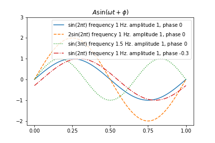
sine function is a simplest form of sound data
- amplitude : $A$
- frequency : $\omega$
- phase : $\phi$
sine expression
- $A \operatorname*{sin}(\omega t - \phi)$
- or
- $A \operatorname*{sin}(2 \pi f t - \phi)$
Frequence is the number of occurrences of a repeating event per unit of time
- $w = 2 \pi f$
- f = 1.0 Hz, T = 1.0 S

import numpy as np
import matplotlib.pyplot as plt

t = np.linspace(0, 1, 100)

plt.plot(t, 1 * np.sin(2 * np.pi * t + 0), ls="-", label=r"$\sin\left(2\pi{t}\right)$ frequency 1 Hz. amplitude 1, phase 0")
plt.plot(t, 2 * np.sin(2 * np.pi * t + 0), ls="--", label=r"$2\sin\left(2\pi{t}\right)$ frequency 1 Hz. amplitude 1, phase 0")
plt.plot(t, 1 * np.sin(3 * np.pi * t + 0), ls=":", label=r"$\sin\left(3\pi{t}\right)$ frequency 1.5 Hz. amplitude 1, phase 0")
plt.plot(t, 1 * np.sin(2 * np.pi * t - 0.3), ls="-.", label=r"$\sin\left(2\pi{t}\right)$ frequency 1 Hz. amplitude 1, phase -0.3")
plt.ylim(-2.2, 3)
plt.xticks(np.linspace(0, 1, 5))
plt.legend()
plt.title(r"$A\sin\left(\omega{t}+\phi\right)$")
plt.show()

wav_data

The relation between frequency and period

$\omega$ : frequency
$T$ : period
$\omega = \frac{2\pi}{T}$

Single Tone

Frequency is tone in human
- tone == beep
- ex) ring tone = 400Hz

def single_tone(frequency, rate=44100, duration=1):
    t = np.linspace(0, duration, int(rate))
    y = np.sin(2 * np.pi * frequency * t)
    return y

y = single_tone(400)
from IPython.display import Audio, display
display(Audio(y, rate=44100))
# You cannot listion tone by your mac

Middle C is 261.65 Hz single tone in the scale
semitone (half tone, half step) $2^{\frac{1}{12}}$

notes = 'C, C#, D, D#, E, F, F#, G, G#, A, A#, B, C'.split(',')
freqs = 220. * 2**(np.arange(3, 3 + len(notes)) / 12.)
notes = list(zip(notes, freqs))
notes
octave = np.hstack([single_tone(f) for f in freqs])
display(Audio(octave, rate=44100))

Wave file format

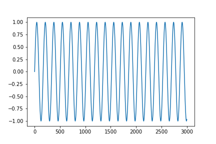
wave file is basic sound pressure time series file format which extension is .wav
wave file usually measure 44100 sound pressure per second and record as 2 bytes between -32768 ~ 32768 $(=2^{15})$
In python, to read or write wave file use read, write command which io.wavfile provide subpakage of scipy package

import scipy.io.wavfile
scipy.io.wavfile.write("octave.wav", 44100, octave)
#octave is exist above code

sr, y_read = scipy.io.wavfile.read("octave.wav")
plt.plot(y_read[:3000])
plt.show()

Audio(y_read, rate=sr)

wav_data

Dual-tone multi-frequency signaling

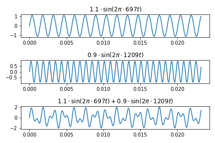
Telephone use the way DTMF(Dual-tone multi-frequency) sound signal the combination of two single-tone to receive telephone number
DTMF is sin + sin

Fourier Transform(FT) and spectrum

Learn about the Fourier transform and spectrum, which are methods of extracting features from speech, music, and sound data

Sine wave combination

Signal can be represented by the combination of frequency, magnitude, phase and other sinusolida signal
The Fourier transform is a method of separating the sinusoids that make up the signal from the combined signal

N = 1024
T = 1.0 /44100.0
f1 = 697
f2 = 1209
t = np.linspace(0.0, N*T, N)
y1 = 1.1 * np.sin(2 * np.pi * f1 * t)
y2 = 0.9 * np.sin(2 * np.pi * f2 * t)
y = y1 + y2

plt.subplot(311)
plt.plot(t, y1)
plt.title(r"$1.1\cdot\sin(2\pi\cdot 697t)$")
plt.subplot(312)
plt.plot(t, y2)
plt.title(r"$0.9\cdot\sin(2\pi\cdot 1209t)$")
plt.subplot(313)
plt.plot(t, y)
plt.title(r"$1.1\cdot\sin(2\pi\cdot 697t) + 0.9\cdot\sin(2\pi\cdot 1209t)$")
plt.tight_layout()
plt.show()

freq_plus_operation

Complex exponential function

By Euler’s formular, complex exponential function with imaginary number in exponential can be represented like below

$exp(i \cdot x) = \operatorname{cos}x + i \operatorname{sin}x$

Fourier Transform

All cyclic function with period T can be represented below

$y(t) = \sum_{k= -\infty}^{\infty} A_{k} exp(i \cdot 2\pi \frac{k}{T}t)$ $A_{k} = \frac{1}{T} \int_{-\frac{T}{2}}^{\frac{T}{2}}f(t) exp(-i \cdot 2\pi \frac{k}{T}t)$

Discrete Fourier Transform

When there are time series data with legnth N

$y_0, y_1,...,y_{N-1}$

DFT suppose repeat N and do FT
In case, discrete time series data is represented below

$y_n = \frac{1}{N} \sum_{k=0}^{N-1}Y_k \cdot exp(i \cdot 2 \pi \frac{k}{N}n)$ $Y_k = \sum_{n=0}^{N-1} y_n \cdot exp(-i \cdot 2 \pi \frac{k}{N}n)$

Fast Fourier Transform (FFT)

Fast Fourier Transform is an algorithm for doing DFT with very little computation
It can be applied in time series with length $2^N$
Big O
- DFT
  - $O(N^2)$
- FFT
  - $O(N\log_{2}{N})$
Gibbs phenonmenon : If the begining and end of time series is too diff, it could create signal which doesn’t exist before

y2 = np.hstack([y, y, y])

plt.subplot(211)
plt.plot(y2)
plt.axvspan(N, N * 2, alpha=0.3, color='green')
plt.xlim(0, 3 * N)

plt.subplot(212)
plt.plot(y2)
plt.axvspan(N, N * 2, alpha=0.3, color='green')
plt.xlim(900, 1270)

plt.show()

freq_plus_operation_check

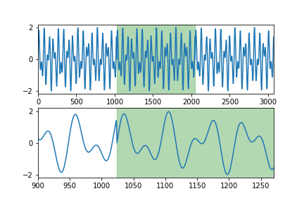
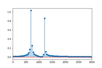
Analysis above frequency with fftp command of scipy.fftpack emphasize 692Hz, 1211Hz
periodgram

from scipy.fftpack import fft

yf = fft(y, N)
xf = np.linspace(0.0, 1.0/(2.0*T), N//2)

plt.stem(xf, 2.0/N * np.abs(yf[0:N//2]))
plt.xlim(0, 3000)

plt.show()

fft

Discrete Cosine Transform

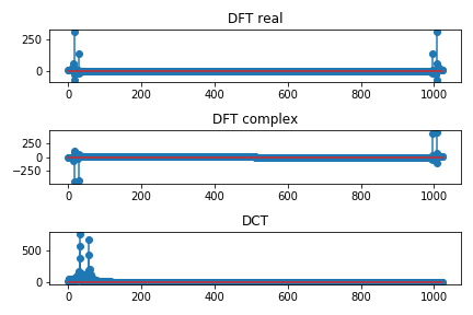
DCT is similar with DFT
basis function is cosine function, not a complex exponential function
Little computation than DFT and print $R$

$Y_k = \sum_{n=0}^{N-1}y_n \cdot cos(2\pi\frac{k}{N}(\frac{2n+1}{4}))$

from scipy.fftpack import dct

dct_type = 2
yf2 = dct(y, dct_type, N)

plt.subplot(311)
plt.stem(np.real(yf))
plt.title("DFT real")

plt.subplot(312)
plt.stem(np.imag(yf))
plt.title("DFT complex")

plt.subplot(313)
plt.stem(np.abs(yf2))
plt.title("DCT")

plt.tight_layout()
plt.show()

dct

Spectrum

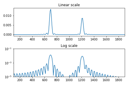
In time series analysis, spectrum is power spectrum or spectral density
The Fourier transform is the transformation of the deterministic time series data into the frequency domain, while the spectrum is the transformation of the stochastic stochastic model into the frequency domain
Unlike the Fourier transform, time-phase phase information does not appear in the spectrum
One of the methods used to estimate the spectrum is to divide the entire time series into short intervals, and then window each interval to reduce the Gibbs phenomenon and average the values from the FFT calculation. Usually expressed in log scale

import scipy.signal

f, P = scipy.signal.periodogram(y, 44100, nfft=2**12)

plt.subplot(211)
plt.plot(f, P)
plt.xlim(100, 1900)
plt.title("Linear scale")

plt.subplot(212)
plt.semilogy(f, P)
plt.xlim(100, 1900)
plt.ylim(1e-5, 1e-1)
plt.title("Log scale")

plt.tight_layout()
plt.show()

periodogram

STFT

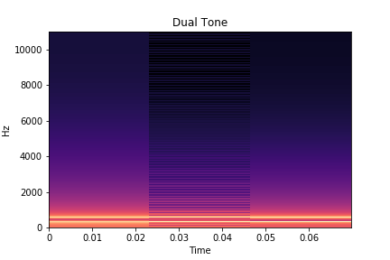
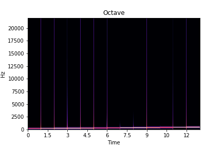
STFT is a method for analyzing sound whose frequency characteristics vary over time
The data is obtained by dividing the time series into regular time intervals and obtaining the spectrum for each interval
Represented as two-dimensional data of time-frequency

librosa Package

Use the librosa package for STFT spectrum analysis in Python
When using the librosa package on Jupyter notebooks, set the iopub_data_rate_limit setting in the jupyter_notebook_config.py file to as large as 10000000

import librosa
import librosa.display

D = np.abs(librosa.stft(y))
librosa.display.specshow(librosa.amplitude_to_db(D, ref=np.max), y_axis='linear', x_axis='time')
plt.title('Dual Tone')
plt.show()

librosa_stft

sr_octave, y_octave = scipy.io.wavfile.read("octave.wav")

D_octave = np.abs(librosa.stft(y_octave))
librosa.display.specshow(librosa.amplitude_to_db(D_octave, ref=np.max), sr=sr_octave, y_axis='linear', x_axis='time')
plt.title('Octave')
plt.show()

specshow

Mel Spectrum

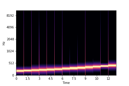
Mel spectrum refers to a spectrum in which units of frequency are converted into mel units according to the following formula
$m = 2595 \operatorname{log}_{10}( 1 + \frac{f}{700})$

S_octave = librosa.feature.melspectrogram(y=y_octave, sr=sr_octave, n_mels=128)
librosa.display.specshow(librosa.power_to_db(S_octave, ref=np.max), sr=sr_octave, y_axis='mel', x_axis='time')
plt.show()

melspectrogram

MFCC

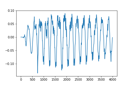
y, sr = librosa.load(librosa.util.example_audio_file())

plt.plot(y[1000:5000])
plt.show()

example_audio

from IPython.display import Audio, display
Audio(y, rate=sr)

S = librosa.feature.melspectrogram(y=y, sr=sr, n_mels=128)
librosa.display.specshow(librosa.power_to_db(S, ref=np.max), sr=sr, y_axis='mel', x_axis='time')
plt.show()

melspectrogram_eaxmple

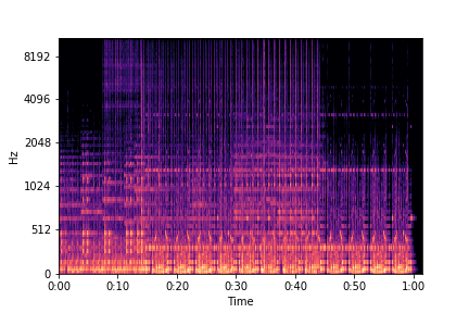
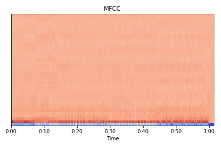
Mel-frequency cepstral coefficients is a coefficient obtained by grouping Mel Scale Spectrum into 40 frequency bands and then Fourier transforming them
It can be thought of as a characteristic value indicating how the spectrum is shaped

mfccs = librosa.feature.mfcc(y=y, sr=sr, n_mfcc=40)
librosa.display.specshow(mfccs, x_axis='time')
plt.title('MFCC')
plt.tight_layout()
plt.show()

mfcc

Digital Sound Processing 01

run to asr